
")
UAP sightings cluster where the seafloor drops fastest.
Recently I posted Phase 1. UAP reports cluster near submarine canyons, even after controlling for population. I tried to challenge it. Maybe the signal is just coastal density the controls didn’t catch?
So I ran four additional analyses, each attacking the population confound differently. Here’s what I found.
The short version
1. The signal survives, but it’s sharper than I thought.
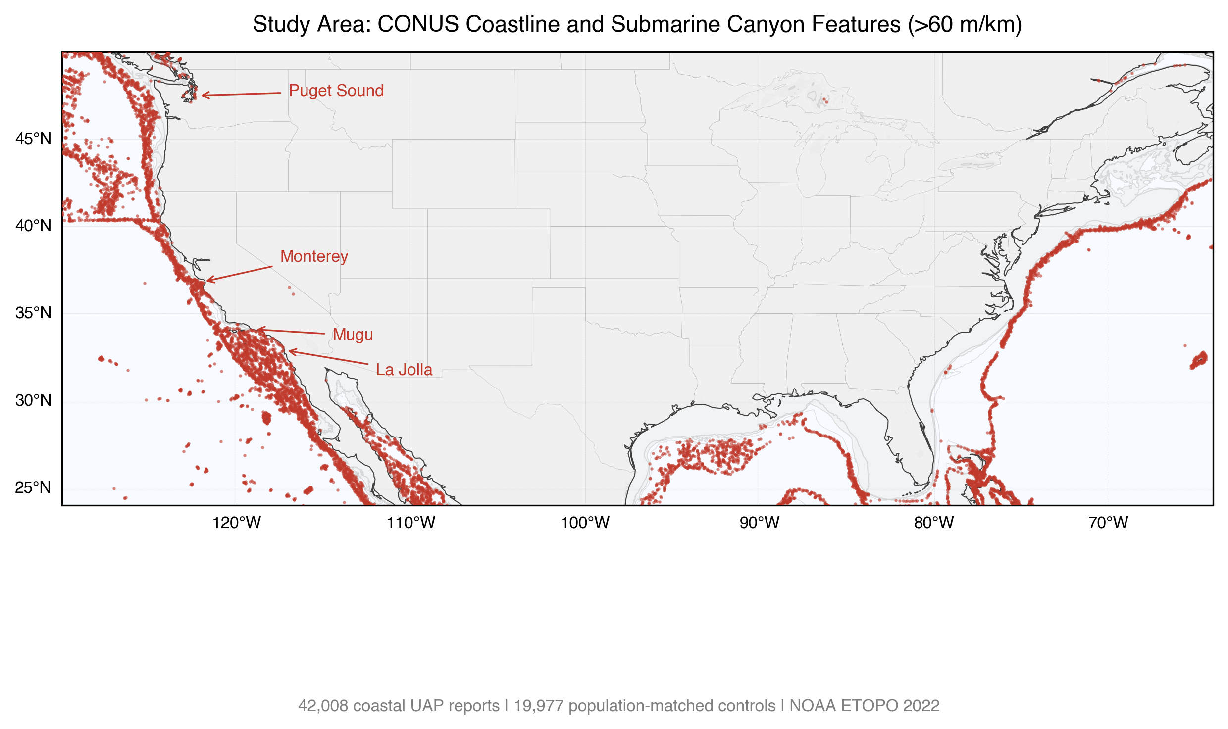
Phase 1 detected canyon cells using a 20 m/km gradient threshold and found odds ratios of 3–5× against population-matched controls. Phase 2 breaks that range into steepness bins, and only the steepest (60+ m/km, which maps to 85% of actual mapped submarine canyons) survives finer-grained population controls. Below that steepness, the signal disappears. Above it: odds ratio 3.90 [1.42–10.83], meaning reports are roughly 4× more likely near steep canyons than expected.
That’s lower than Phase 1’s headline OR of 5.30, because Phase 2 uses more conservative population controls that work at sub-county resolution instead of county level. The effect is real but smaller than it first looked. Maybe closer to something that actually makes sense.
2. It’s not just spatial. It’s also temporal.
Reports near canyons also cluster in time. Not a steady background hum. Episodic bursts. A few reports in the same area within days of each other, then nothing. I found 61 such clusters. The top 5 are all within 10 km of a canyon: three in Puget Sound, two in Southern California. Specific coordinates and dates in the repo.
What changed from Phase 1?
| Phase 1 | Phase 2 | |
|---|---|---|
| Main finding | Reports cluster near canyons | Only near steep canyons, in episodic bursts |
| Canyon threshold | 20 m/km (all canyon cells) | 60+ m/km (true canyon features only) |
| Odds ratio | 5.30 at 10 km (county-matched) | 3.90 at 60+ m/km (finer population controls) |
| Effect type | Smooth distance decay | Binary threshold + temporal clusters |
| Population control | County-level matching | Finer-grained sub-county controls |
| Honest effect size | Large | Smaller but consistent |
Phase 1 showed that spatial association is real and survives metro removal and placebo shelf tests. Phase 2 sharpens it.
The five flap episodes
The temporal test found 61 spatio-temporal clusters. Here are the top 5:
| # | Reports | Location | Dates | Distance to canyon |
|---|---|---|---|---|
| 1 | 5 | Puget Sound | 2002-10-01 | 1.6 km |
| 2 | 6 | Orange County coast | 2007-10-06 to 10-12 | 8.5 km |
| 3 | 3 | Puget Sound | 2001-10-15 to 10-19 | 8.2 km |
| 4 | 3 | Puget Sound | 2000-10-22 to 10-25 | 1.8 km |
| 5 | 4 | Santa Monica coast | 2010-10-28 to 11-06 | 1.0 km |
These are exact coordinates and date ranges. Checkable against independent records. Full episode map in the repo.
What this doesn’t prove?
The temporal clustering could be social contagion. One person reports something, neighbors look up and report too. The 60+ m/km threshold could be geometric, canyon mouths sit right at the coast where people live, and the controls may not fully capture that. The confidence interval on the odds ratio spans from 1.4 to 10.8, which is almost an order of magnitude. And I can’t control for observer type: fishermen and sailors see different things than suburban residents.
This is a pattern in self-reported data. It measures reporting behavior, not the phenomenon.
What would settle it?
Hydrophones. NOAA passive acoustic arrays sit near Puget Sound, La Jolla, and Monterey. Exactly where the flap episodes concentrate. Underwater, there’s no reporting bias. If anomalous acoustic signatures show up at the same coordinates and dates listed above, the reporting-bias explanation dies.
The flap table gives exact where and when. That’s a testable prediction.
For the technically minded
Full methodology below. Same 42,008 coastal NUFORC reports and 19,977 population-matched controls as Phase 1. All code, data, and intermediate outputs in the repo.
Detailed methodology:
Temporal permutation test
For each report, I find all other reports within 50 km, then count how many fall within ±7 days. The ratio of observed to expected temporal neighbors gives an excess score, normalized for local density. Test statistic: median excess near canyons minus far from canyons. Null: shuffle dates within each calendar year (1,000 iterations) or within each month (200 iterations, stricter).
Within-year: z = 6.18, p < 0.001. Within-month: z = 4.05, p = 0.015.
The signal lives in the tails. Trimming to the 5th–95th percentile reverses the effect (z = −5.32). It’s driven by rare, sharp bursts, not a diffuse background. 10/36 parameter combinations (temporal window × spatial radius × canyon threshold) are significant after FDR correction.
GAM partial dependence
Generalized additive model with 7 covariates: distance to canyon, coast, military bases, population density, ocean depth, port distance, and port count. Thin-plate spline on canyon distance (8 basis functions, AIC-selected). The partial effect spans 2.77 log-odds over 0–300 km, with most of the drop in the first 50 km. GAM beats linear on all metrics (AIC 68,612 vs 68,774, CV AUC 0.675 vs 0.657).
Weighted odds ratios by canyon steepness
Phase 1’s county-matched ORs of 3–5× don’t fully resolve within-county density gradients along canyon coastlines. Importance weighting (1/sampling score) isolates the canyon-specific component at sub-county resolution, with 2,000 bootstrap iterations.
Results: only the 60+ m/km bin (weighted OR 3.90 [1.42–10.83]) excludes 1.0. Lower gradient bins don’t survive weighting. This is a binary threshold, not dose-response.
Phase 1’s county-matched ORs are 2–3× higher across all bins. The difference reflects within-county population gradients. Importance-weighted estimates are the more conservative measure.
Cluster bootstrap
Standard errors assume independence. UAP reports from the same area aren’t independent. Cluster bootstrap (2,000 resamples, 4,057 spatial clusters): β = −0.166, CI [−0.258, −0.074]. The CI is 4.4× wider than naive but still excludes zero.
Per-distance cluster-bootstrapped ORs: 1.21 at 10 km [1.09–1.34], 1.18 at 25 km [1.08–1.29], 1.13 at 50 km [1.06–1.21].
Code, data, and full tables: https://github.com/antoniwedzikowski-rgb/uap-canyon-analysis
Analysis designed by me. Code generated with Claude Code. Writeup edited with AI assistance. I welcome methodological critique.
by Any_Cartographer2016
8 Comments
I tested whether UAP sightings cluster near underwater geological structures using 41k coastal reports, NOAA bathymetry, and Census-matched controls. The signal survives permutation tests and metro removal, but concentrates only at the steepest canyon gradients (>60 m/km). Full methodology and reproducible code are in the repo.
For anyone who prefers audio summaries (like me), I ran the analysis through NotebookLM and recorded a discussion-style walkthrough. It doesn’t add new claims, just explains the methodology in plain language. Link below.
[https://github.com/antoniwedzikowski-rgb/uap-canyon-analysis/blob/main/media/UAP_Sightings_Cluster_Around_Submarine_Canyons.m4a](https://github.com/antoniwedzikowski-rgb/uap-canyon-analysis/blob/main/media/UAP_Sightings_Cluster_Around_Submarine_Canyons.m4a)
Good work and very interesting. I wonder if time of day plays a part as well.
Subterranean quartz experiencing enough seismic fault pressure to cause massive piezoelectric effects strong enough to generate electrostatic luminescent atmospheric phenomena.
“Let me be direct about this.” That would be nice, but it doesn’t happen. It’s hard to take anything this saturated with AI slop writing seriously. But that aside, is there anything else that is more common at these locations, like maybe fishing or oil platforms?
Have you looked at the data in terms of population density, or more specifically, reports generated per average number of observers within each area? This is a great analysis BTW, but I would be interested to know how many large population centers or busy maritime routes happen to be near deep coastal trenches.
Population centers are all near the ocean. Couldn’t it just be most sightings happen where more people are living?
The map correlates strongly to offshore military training ranges.
Well men, only one way to find out! Someone needs to set up several monitoring sensors on a buoy and record the data