

Description of COMET-LF
Figure 1a describes the transmission dynamics of W. bancrofti infection, disease and the impact of MDA as employed in COMET-LF. We consider seven human compartments, namely, susceptible humans (\(S_h\)), exposed humans with L3 larvae (\(E_h\)), those with adult worms (\(W_h\)), asymptomatic infectious humans with Mf and adult worms (\(M_h\)), humans with sterilized adult worms (\(W_{ht}\)), humans with symptomatic disease (\(D_h\)) and individuals who achieved clearance of adult worms and Mf (\(C_h\)). The \(D_h\) compartment represents the combined burden of humans with lymphoedema or hydrocele. We adopt this simplifying assumption, as the pathogenesis, onset times and treatment responses of these two forms of clinical manifestations are not clearly understood. While the progression of infected persons to hydrocoele may be associated with worm burden, progression to lymphoedema is due to immunopathological reactions and secondary bacterial infections [34]. However, a recent review reported that immune response plays a crucial role in the progression of both lymphoedema and hydrocele [35]. Within our model, we consider the total human population of the system at any given time t to be \(N_h(t)=S_h(t)+E_h(t)+W_h(t)+M_h(t)+W_{ht}+D_h(t)+C_h(t)\). Susceptible humans become exposed through the bite of an infected female mosquito at a rate \(\lambda _{vh}\) and move to the \(E_h\) compartment. The force of infection from mosquitoes to humans, \(\lambda _{vh}\), is assumed to be the product of the average mosquito bites per human per unit time \(\beta \frac{N_v(t)}{N_h(t)}\), the probability that the mosquito is infected \(\frac{I_v(t)}{N_v(t)}\), and the probability of successful transmission of infection from vector to human \(\theta _{vh}\), i.e. \(\lambda _{vh} = \beta \theta _{vh}\frac{ I_v(t)}{N_h(t)}\). Susceptible humans also increase at a rate \(\Pi _h\) due to recruitment through new births. Exposed humans may achieve clearance of the L3 larvae at a rate \(\omega _E\) and move to the \(C_h\) compartment. Else, the L3 larvae can grow to become adult worms and thus a human in the \(E_h\) compartment may transfer to \(W_h\) compartment at rate \(\lambda _E\). From \(W_h\), individuals can achieve clearance (rate \(\omega _W\)), or transfer to \(M_h\) at a rate \(\lambda _W\) if adult worms mate to produce Mf. Both humans with a history of adult worms and Mf can develop symptomatic disease (lymphoedema or hydrocele). We assume humans in the \(W_h\) compartment can move to \(D_h\) at a rate \(\alpha _1\), while humans in the \(M_h\) class move to \(D_h\) at a rate \(\alpha _2\). Humans who have achieved clearance of adult worms and Mf are assumed to have temporary immunity to reinfections. Humans in the \(C_h\) compartment lose immunity at a rate i and become susceptible again. We assume that all the human compartments decrease due to natural death at rate \(\mu\). The natural birth and death rates were taken from the Sample Registration System [36] for Bihar.
Fig. 1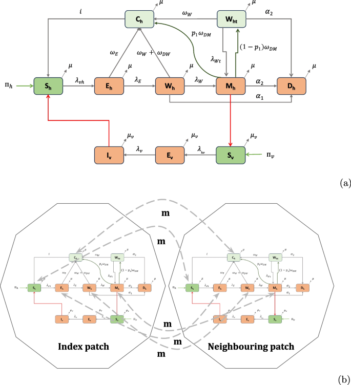
a Flow diagram of COMET-LF. Susceptible humans (\(S_h\)) become infected with L3 larvae (\(E_h\)) through bites of infectious mosquitoes (\(I_v\)). They can either self-clear L3 (\(C_h\)), or become hosts to adult worms (\(W_h\)). Adult worms can mate to produce microfilaria (\(M_h\)). Susceptible mosquitoes (\(S_v\)), which take a blood meal from these humans, become exposed (\(E_v\)) and eventually become infectious. Humans with a history of adult worms or Mf can develop symptomatic disease (lymphoedema or hydrocele), represented in compartment \(D_h\). MDA effects are modeled through additional cure rates \(\omega _{DW}\) and \(\omega _{DM}\) of the \(W_h\) and \(M_h\) compartments and by incorporating an additional compartment for people with sterilized adult worms (\(W_{ht}\)). In the absence of MDA, these two rates as well as the \(W_{ht}\) compartment are set to zero. b Schematic representation of the two-patch system. Humans in all compartments, except the disease compartment, migrate between the two patches with rate m
The vector population is divided into 3 epidemiological compartments: susceptible vectors (\(S_v\)), exposed vectors with Mf (\(E_v\)), and infectious vectors (\(I_v\)) (Fig. 1a). Therefore, the total vector population at any given time t is \(N_v(t) = S_v(t) + E_v(t) + I_v(t)\). Susceptible mosquitoes become exposed when engorging on the blood of infectious humans at a rate \(\lambda _{hv}\). The force of infection from humans to mosquitoes is \(\lambda _{hv} = \beta \theta _{hv}\frac{M_h(t)}{N_h(t)},\) which is the product of the average number of bites per mosquito per unit time \(\beta\), the probability that the human is infectious \(\frac{M_h(t)}{N_h(t)}\), and the probability of successful transmission of infection from human to vector \(\theta _{hv}\). Additionally, susceptible mosquitoes are recruited at a rate \(\Pi _v\) due to new births. Exposed mosquitoes may become infected at a rate \(\lambda _v\). We assume that all mosquito classes decrease due to natural death at a rate \(\mu _v\).
An important intervention in the context of LF elimination is MDA. We investigate the effect of MDA in our model for different baseline scenarios of Mf prevalence. MDA campaigns are conducted annually, and we incorporate this through a time-dependent impulsive MDA function \(\gamma (t)\). If \(t_{MDA_i}\) is the first week of conducting \(i^{th}\) MDA, then the impulsive MDA function is given by,
$$\begin{aligned} \gamma (t) = \left\{ \begin{array}{ll} \text {(MDA coverage)/4,} & \quad \text {if} \quad t_{MDA_i} \le t \le t_{MDA_i} + 3\\ 0, & \quad \quad \text {otherwise} \end{array}\right. \end{aligned}$$
This approach is consistent with existing EPIFIL and LYMFASIM models, which also consider MDA activities conducted in a particular month of a given year [37]. Infectious humans (\(M_h\)) are assumed to clear Mf at a rate \(p_1 \omega _{DM}\) due to MDA and move to \(C_h\). Individuals from \(M_h\) also move to \(W_{ht}\) at a rate \((1-p_1) \omega _{DM}\) due to MDA. Similarly, humans with adult worms but no Mf (\(W_h\)) move to \(C_h\) at a rate \(\omega _{DW}\) due to MDA. We assume \(\omega _{DM} = p_2 \gamma (t)\), and \(\omega _{DW} = p_1 \gamma (t)\), where \(p_2\) models the effect of the drug on clearing Mf (proportion of persons cured from Mf), while \(p_1\) is the effect of the drug on adult worms (proportion of persons that cleared adult worms). We consider both the DA and IDA drug regimens for simulation. We use human clinical trial data in the Indian setting to model the effects of MDA in the COMET-LF model. For DA and IDA, the value for \(p_1\) is taken as 15% [14] for both the drug regimens while values of \(p_2\) are taken as 61.8% and 84%, respectively [14]. This approach is in contrast to EPIFIL and LYMFASIM which models MDA effects by considering the percentage of Mf clearance, percentage of worms killed and worm sterilisation periods as reported in Irvine et al. [37]. Additionally, we consider the worm sterilization period due to DA and IDA are 1 year and 5 years respectively [38, 39]. The parameter \(\lambda _{Wt}\) is considered accordingly as \(\frac{\lambda _W}{\text {Sterilization period}}\) for DA and IDA.
The mathematical equations governing the dynamics of infection are detailed in Supplementary Information (SI) 1A text. The description of model parameters and their corresponding estimates from published literature or expert opinions are reported in Table 1.
Table 1 Fixed model parameter descriptions and their estimates from literature
For the COMET-LF model without MDA effect, we derive the expression of the unique disease-free equilibrium (DFE) of the model. Using the next-generation matrix method [41], we calculate the basic reproduction number (\(R_0\)) as follows:
$$\begin{aligned} R_0 = \sqrt{\frac{\beta \theta _{vh} \lambda _E \lambda _W }{ \Pi _h(\omega _E + \lambda _E+\mu )(\omega _W +\lambda _W + \alpha _1 + \mu )} \times \frac{\beta \theta _{hv} \lambda _v \Pi _v }{\mu _v^2(\lambda _v + \mu _v)}}. \end{aligned}$$
(1)
The square of the basic reproduction number \(R_0\) is a product of two terms. The first term consists of parameters related to human compartments while the second term has parameters from mosquito-related compartments. The first term indicates the number of susceptible mosquitoes infected by a single infectious human. The second term, in turn, indicates the number of susceptible humans that will be infected by an infectious mosquito, and the product of these gives a measure for \(R_0\) [42].
Using dynamical system theory, we prove that the DFE of the model (S1) is globally asymptotically stable whenever \(R_0. We also calculate the endemic equilibria (EE) and their local stability conditions. The proofs of these analytical results are given in SI 1B and SI 1C text.
The model equations corresponding to MDA implementation in COMET-LF is provided in SI 1D text.
Model calibration and scenario analysis
We calibrate the model in the absence of MDA (\(\omega _{DM} = \omega _{DW} = 0\)) using publicly available annual Mf rates and symptomatic disease rates for Bihar for the period 2008–2013 from Indiastat [43]. In the calibration step, we estimate seven parameters – the probability of successful transmission of infection from vector to human \(\theta _{vh}\), the progression rate from humans with L3 larvae to humans with adult worms \(\lambda _E\), the self-cure rate of exposed humans in absence of MDA \(\omega _E\), the rate at which humans with adult worms develop Mf \(\lambda _W\), the self-cure rate of humans with adult worms in absence of MDA \(\omega _W\), and the two disease progression rates \(\alpha _1\) and \(\alpha _2\) from the \(W_h\) and \(M_h\) compartments, respectively. All the rates are allowed to vary in the interval (0, 1), while \(\theta _{vh}\) lies in the range (0, 0.37) [20]. We calibrate time series data using the MATLAB function ’fminsearchbnd’ to minimise the sum of squared error between baseline and model-generated outputs of Mf rate and disease rate. The estimates of \(\alpha _1\) and \(\alpha _2\) remain unchanged throughout the rest of the paper. Table 1 shows the list of known parameters for which estimates are taken from the literature.
To validate the model predictions, we considered programmatic data of Mf prevalence from 10 endemic districts in Bihar in 2018 and 2019. Each district had data from eight sites (four sentinel and four random sites). These were averaged to obtain the mean and the standard deviation of the Mf rate for each district. We used the 2018 data to calibrate our model to the observed Mf rate for each district. In this process, we estimate 5 parameters as described at the beginning of this section. We then used programmatic estimates of MDA coverage, and the estimated parameter set, to predict the Mf rate in 2019.
For the scenario analysis, the calibrated model was applied to simulate different MDA-scenarios (2 drug regimens, 5 levels of MDA coverage: 45%, 55%, 65%, 75% and 85%) for four different endemic scenarios (1.5%, 2%, 5% and 10%). Thus, 10 MDA scenarios were simulated for each endemic scenario. MDA coverage ranges were chosen based on the previous studies and programmatic estimates. IDA coverage in urban districts can become as low as 38% [13]. According to NCVBDC, the administrative IDA-MDA coverage at the district level can be as high as 95%. This is also consistent with MDA coverage ranges of previous modeling studies [37]. We varied 5 parameters so that the model-generated Mf rates match with the four endemic scenarios. The parameters are \(\theta _{vh}\), \(\lambda _E\), \(\omega _E\), \(\lambda _W\) and \(\omega _W\). All the rates were allowed to vary in the interval (0, 1), while \(\theta _{vh}\ \epsilon \ (0,0.37)\) [20]. We produced 100,000 initial samples using Latin Hypercube Sampling. For each baseline scenario, we identified 250 samples that fall within the required Mf rate with an allowable error of \(\pm 0.5\%\) (e.g. 1% – 2% for the 1.5% baseline). We identified samples of parameters that lead to the baseline Mf rates 1.5% (1% – 2%), 2% (1.5% – 2.5%), 5% (4.5% – 5.5%) and 10% (9.5% – 10.5%). The identified samples were then used to generate future trends of Mf rates using the model. The number of MDA rounds required to achieve
Impact of MDA on disease (lymphoedema and hydrocele) prevalence
Using the previously obtained equilibrium fits to different levels of baseline Mf rates, \(10\%\) and \(2\%\) (Model calibration and scenario analysis section), we simulated 6 scenarios to assess the impact of 5 annual rounds of MDA (DA or IDA) for 3 different MDA coverages (45%, 65% and 85%). We predicted the trends in disease prevalence over time before and after stopping MDA over 20 years.
Implementation of EPIFIL and LYMFASIM
We applied both EPIFIL and LYMFASIM to simulate the impact of a single dose of DA and IDA, administered annually, for different MDA-scenarios considered in COMET-LF. For both models, we used the respective model estimates for all the biological parameters, representing Indian settings, as described elsewhere [20, 44]. While in LYMFASIM we allowed the mosquito biting rate to vary from 1600 to 3200 per month to represent different endemic scenarios in India, in EPIFIL, we followed the same methodology as COMET-LF to simulate the different endemic scenarios.
In both LYMFASIM and EPIFIL, the efficacy of the drug regimens, DA and IDA, are distinguished by 3 different parameters – worm killing rate, worm sterilisation rate, and Mf clearance rate (Table 2). For both these models, drug efficacies were obtained from Irvine et al. [37]. For each scenario: baseline Mf rate (1.5%, 2%, 5% and 10%), MDA-coverage (45%, 55%, 65%, 75% and 85%), and for a fixed round of either DA or IDA, 1000 simulations were conducted. The number of simulations in which an Mf rate was found
Table 2 Two drug regimens and their corresponding effects on Mf clearance rate, worm killing rate, and worm sterilisation rateMetapopulation model for migration
Metapopulation models have been used in the literature to investigate the effects of migration [45]. In this approach, the population is partitioned into a number of discrete patches or regions. In each region, the disease dynamics follows a compartmental model corresponding to the infection and disease prevalence in this region. Humans can migrate between the distinct regions, leading to a multi-patch multi-compartment model of disease transmission. For our metapopulation model (model description in SI 1F), we consider a two-patch system to investigate the role of migration. We assume that the two patches are connected through migration of susceptible humans, exposed humans, people with adult worms, people with both adult worms and Mf, and cured people. We introduce a migration rate parameter (m) for all the classes of humans. For simplicity, we assume the migration rates of all the classes are the same. A schematic of this model is shown in Fig. 1b.
The migration rate m is calculated based on 2011 census (D-02 series [36]) data for migration within and across states in India. The in- and out-migration rate of Bihar is estimated using the current, last place of residence and all duration of residence data [36]. The in-migration and out-migration rates per 1000 population per 10 years are calculated as:
$$\begin{aligned} \text {In-migration rate} = \frac{\text {Volume of in-migration to the state} \times 1000}{\text {Enumerated population of the destination state}} \end{aligned}$$
and
$$\begin{aligned} \text {Out-migration rate} = \frac{\text {Volume of out-migration from state} \times 1000}{\text {Enumerated population of the state of origin}}. \end{aligned}$$
For Bihar, the value of in-migration and out-migration are 11 per 1000 and 72 per 1000, respectively. We use the mean value of these to obtain the migration rate of \(m= \frac{(72+11)}{2 \times 1000 \times 52 \times 10} = 0.00008\) per week for Bihar. To account for demographic changes and temporary migration for seasonal work, we also simulate the model for 2 higher migration rates, \(m=0.0005\) and \(m=0.001\). All other parameters are taken from Table 1 and MDA related parameter values are taken from the Description of COMET-LF section.
For the simulations that compute additional number of MDA rounds, we consider that the index (or target) location is connected to a neighbouring region, each with its own baseline Mf rate \(\in \{1.5\%, 2\%, 5\%, 10\%\}\). The value of the migration parameter is assumed to be 0.001. We apply MDA to both regions with a coverage of \(45\%\). Among the 250 \(\times\) 250 parameter values and initial conditions, we simulate the metapopulation model with 100 \(\times\) 100 parameter values and initial conditions. Based on the number of MDA rounds predicted for the given baseline Mf rate in the absence of migration in the neighbouring patch, we calculate the required number of MDA rounds to achieve elimination in the target location. For the simulations, which investigate the risk of resurgence in a non-endemic region, we consider the target location to be an infection-free patch where all humans and vectors are susceptible and couple it to a neighbouring location with a baseline Mf rate of 1.5%, 2%, 5% or 10%. We assume that all disease-related parameters and the total population are the same in both patches. We consider 3 different migration rates, 0.001, 0.0005 and 0.00008, for all the trajectories. We then calculate the risk of Mf transmission in the non-endemic patch by dividing the number of trajectories >1% Mf rate after 5 years in the disease-free block by the number of all trajectories.